Solver optimization for strong coupling of DC and HT

Hey guys,

I am working on a problem which features a strong dependence of temperature and conductivity.

A ceramic heating element is heated through Joule heating. As the ceramic is a PTC, the electrical conductivity increases rapidly once the temperature passes a certain threshold (the so-called Curie-temperature).
I have successfully modeled the behavior of the electrical conductivity in dependence of the temperature through the following function:

R = (T<=T_curie)*R_0 + (T>T_curie)*R_0*(1+(T-T_curie)^Curie_exp)
sigma = 1/R

Bascially, the resistance increases by 10e2 over about 5K, once it goes past T_curie.

The challenge: Once the simulation reaches the point where the resistance is no longer constant, it becomes very unstable. I understand that this is mainly caused by the very strong interaction between

V -> Q -> T -> R -> V

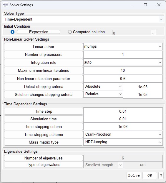
I have been able to tackle this with a high relaxation factor of 0.6 and a timestep of 0.01, but this makes the simulation very slow, especially as the small timestep is not necessary for the part where R stays constant.

Any suggestions on how I could further optimize the solver?

I have read a couple of things about variable time-stepping or relaxation factors decreasing between iterations, but I don't think I can implement those through the GUI.

I would gladly attach the model, but I don't know how to delete the results from the file and with them it is too big. But here are at least the current solver settings.

This is kind of tricky. You seem to have played with the most relevant parameters. Some other factors that can be used to speed up simulations:

  - Simplify geometry by utilizing symmetry
  - Reducing mesh size (or optimizing mesh)
  - Reduce (finite) element shape function order (if using higher order >= 2)
  - Reduce defect/solution changes stopping criteria (tolerance)

You might also try switching to the more robust but 1st order, "Backward-Euler" time stepping scheme.

Other than that one would probably want to write a custom solver m-file script for this, perhaps using values from the old time step in each iteration to compute "R" and "sigma".

Lastly, if you know "T_curie" happens at a specific time and it doesn't fluctuate, you might try to split the computation in two parts 0 < t(T_curie) and t(T_curie) < t_end.

Edit: You might also give the FEniCS solver a try. The built-in solver employes simple 1st order (Picard) iterations for linearization of non-linear problems, while FEniCS employ analytic derivation and the Newton method which theoretically should lead to faster (2nd) order convergence but might be more sensitive (without a good initial guess).