Smoothed Results


|
Other FEA software I have used had selections for post processing that included the word "smoothed". I observed that the results - especially evident in the iso lines - for the smoothed vs non-smoothed indicated some sort of modification of the result data so as to "curve fit" it giving a smooth vs jagged appearance.
Is there such a feature available in the FEAtool? Since FEAtool will export the fea struct, could the result could be processed and replaced by "smoothed" data, and then postplot'ed? Could the Matlab smoothX functions be used for this? Kind regards, Randal |
|
Administrator
|
FEATool aims as much as possible to show you results "as is", and therefore does not currently feature smoothing of results (FEATool is in fact one of the few, if only, simulation software that can also show discountinous solutions). This effectively might mean that regions with non-smooth results are under-resolved and might require a finer grid. To render a smoothed solution you might want to look in to external postprocessing sofware, such as ParaView. That said, there is another effect involved when visualizing expressions that involve derivatives. By default, FEATool employs first order approximations of the solution variables, which means using a linear polynomial on each grid cell. This naturally results in a piecewise constant evaluation of derivatives which is non-smooth. If these quantities are important, it is better to choose a higher order solution space (by selecting it in the "FEM Discretization" section of the "Equation Settings" dialog box). However, the drawback of using higher-order discretizations is larger problem size (as there now also involves implicit mesh points on edges, faces, and cell centers) leading to higher memory consumption and longer solution time (which is why it is not used by default). |
|
|
This post was updated on .
While I am pursuing the ParaView solution, I am also attempting to produce a second order solution by increasing the "FEM Discretization" that you recommend here: However, when I use the "Equation Settings" to set "sflag2" to refine the "sflag1" results (immediately below): 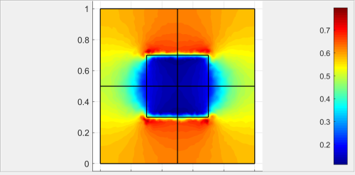 ... I get an unreasonable second order result: 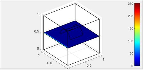 My first thought was perhaps there are some other setting that should also be adjusted while refining results with"FEM Discretization". Then I wondered if the solution had been driven unstable by my inputs and I decided to loosen the grid (fewer points). After doing so, I was able to get the 2nd and 3rd order solutions to solve with smoother lines each time (plotting iso line contours using PareView. Here are the plots for 1st, 2nd, and 3rd order solutions: 1st Order (sflag1): 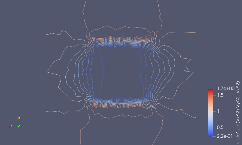 2nd Order (sflag2): 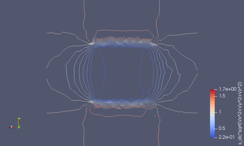 3rd Order (sflag3): 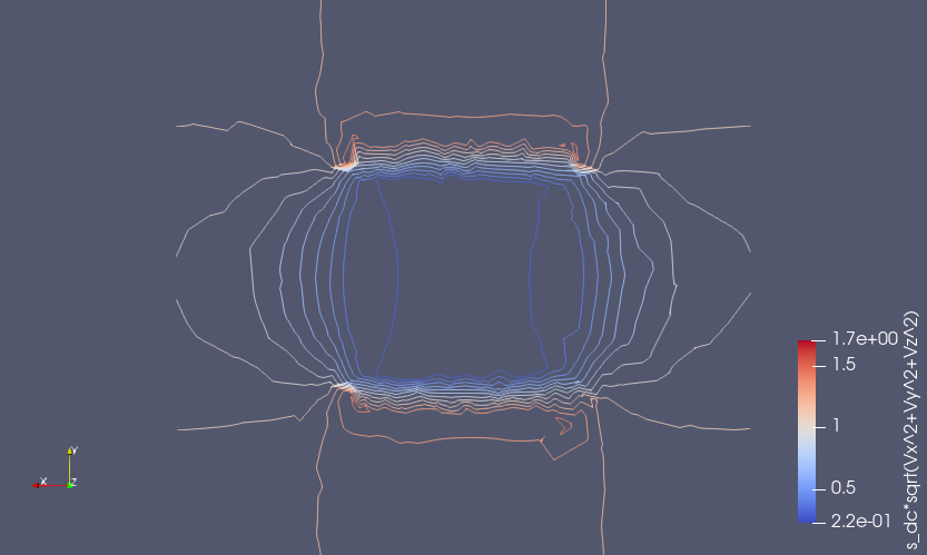 However, I have several questions about the FEM Discretization settings. First, I got the idea from the users guide that each sub-domain could have its own setting: fea.sfun = { ’sflag2’ ’sflag2’ ’sflag2’ };But when I set the discretization for each (e.g., sflag1 for sub-domain 1 and sflag2 for sub-domain 2) it seems that only one was used for the solution. On examination of the exported fea, fea.sfun had only one entry - the last one that was specified. What am I missing? Kind regards, -Randal |
|
Administrator
|
Typically one would not need to adjust much if anything when changing FEM shape functions. In your results it looks kind of like the issue is along the edge of one of the boundaries. This could possibly be due to poor mesh quality (distorted mesh shapes), sometimes it helps to add more "Smoothing" steps in the grid generation process. Although unlikely, it could also be due to numerical under-integration (when building the sparse FEM system matrices), you can try to export your "fea" struct to Matlab and then (re-)solve the model with something like
    fea.sol.u = solvestat( fea, 'icub', 5 );
    postplot( fea, 'parent', figure(), 'sliceexpr', 'V' )
and see if it possibly helps. The shape functions can not be set on a per-subdomain basis (and must thus be the same for all subdomains). The syntax above applies to a problem with three dependent variables (each dependent variable can have a different FEM approximation space). Although certainly technically possible to implement, connecting regions with different shape functions, similar to hanging (non-conforming) grids, mixing and using different mesh cell shapes introduces significant complexeties and would require a significant rewrite of the numeric core. |
|
|
Thanks for the suggestion, but I got the same strange result. However, as I mentioned above, I loosened the grid and then increased the order to 2 and then 3 and got reasonable results. Let's just chalk this one up to a numeric error due to the way I set it up... Understood. I leaped to the wrong conclusion in my reading of the code. Should have read the documentation :-) Before I leave this thread I want to be sure there is nowhere else (within reason) to go within MATLAB/FEAtool in pursuit of smoothed contour/iso lines on a cut-plane/slice. I understand that judicious grid definition and higher order solution space are both avenues within FEAtool that work toward this objective. And I now understand how to better use them. However, by its very piece-wise nature, the FEA solution will not be "smooth" (unless the grid sizes are smaller than the graphic display pixel size :-). So at the expense of accuracy, a contour (iso line) that is an approximation/curve-fit to the solution data can be produced that, although somewhat inaccurate, might still be a reasonable representation of the solution. [BTW, I understand that these contours on slices/cut planes are not a current feature of FEAtool; I can get that from ParaView, however I would like to give to ParaView smoother data, since getting smoothing within ParaView has also eluded me (https://discourse.paraview.org/t/smoothing-contours-iso-lines-on-a-planar-slice/4104 ). See FEAtool forum Basic thread "Slice Plot of 3D Result Showing Iso Contour Lines on a Slice" for further discussion of the contour on slice issue.] I have seen a number of Matlab functions (smooth, smooth3D, smoothdata) that sound like potential solutions. Could the fea solution data be extracted and smoothed and then plotted from Matlab? I am not referring to some large development effort, which of course could be done, but some orchestration of existing functions/scripts that could accomplish the objective. Kind reagards, Randal |
|
Administrator
|
This post was updated on .
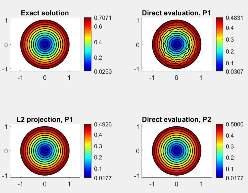
Although technically possible, I don't think smoothing is the right approach here as it will degrade an already low order solution/expression and make it even worse (at least "non-optically"). If the expression you want to evaluate involves gradients and derivatives you can use gradient recovery techniques, here below is an example of using a basic L2 projection FEM approach, which essentially consits of solving
\[ \mathbf{M}u_{x_i} = \mathbf{B}_{x_i}u \] where $\mathbf{M} = \int_\Omega \phi\psi\ d\Omega$ is the (lumped) mass matrix, $\mathbf{B}_{x_i} =\int_\Omega \frac{\partial \phi}{\partial x_i}\psi\ d\Omega$ a gradient matrix in the corresponding direction, $\phi$ and $\psi$ the FEM test and trial functions, and $u$ the known nodal solution vector. More advanced techniques such as polynomial preserving recovery (PPR) [1] and ZZ- recovery [2,3] is also possible but would require custom code.
    % Example of computing/recovering gradients via L2 projection and
    % comparison with direct differentiation of FEM solutions with P1
    % and P2 finite element Lagrange shape functions.

    % Poisson equation on a unit circle with first order P1 basis functions.
    fea = ex_poisson2( 'sfun', 'sflag1', 'iplot', false );

    % (1) Plot exact solution of "sqrt(ux^2+uy^2)".
    f = figure();
    subplot(2,2,1)
    exact_solution = 'sqrt( x^2/2 + y^2/2 )';
    postplot( fea, 'parent', f, 'surfexpr', exact_solution, 'isoexpr', exact_solution, 'isomap', 'k' )
    title('Exact solution')

    % (2) Plot computed solution, P1.
    subplot(2,2,2)
    gradu_expr = 'sqrt(ux^2+uy^2)';
    postplot( fea, 'parent', f, 'surfexpr', gradu_expr, 'isoexpr', gradu_expr, 'isomap', 'k' )
    title('Direct evaluation, P1')

    % Compute L2 projection of ux and uy.
    fea_L2 = fea;
    fea_L2.eqn.m.form{1} = [1;1];
    fea_L2.eqn.m.coef{1} = {1};
    fea_L2.eqn.a.form{1} = [2;1];
    fea_L2.eqn.a.coef{1} = {1};

    [M,Bx] = assembleprob( fea_L2, 'f_m', true, 'f_a', true, 'f_sparse', true );

    fea_L2.eqn.a.form{1} = [3;1];

    [~,By] = assembleprob( fea_L2, 'f_a', true, 'f_sparse', true );

    ux = M\(Bx*fea_L2.sol.u);
    uy = M\(By*fea_L2.sol.u);

    gradu_L2_P1 = sqrt( ux.^2 + uy.^2 );
    fea_L2.sol.u = gradu_L2_P1;

    % (3) Plot L2 projected solution.
    subplot(2,2,3)
    postplot( fea_L2, 'parent', f, 'surfexpr', 'u', 'isoexpr', 'u', 'isomap', 'k' )
    title('L2 projection, P1')

    % Poisson equation on a unit circle with second order P2 basis functions.
    fea_P2 = ex_poisson2( 'sfun', 'sflag2', 'iplot', false );

    % (3) Plot computed solution, P2.
    subplot(2,2,4)
    postplot( fea_P2, 'parent', f, 'surfexpr', gradu_expr, 'isoexpr', gradu_expr, 'isomap', 'k' )
    title('Direct evaluation, P2')
 [1]: Z. Zhang, Polynomial preserving gradient recovery and a posteriori estimate for bilinear element on irregular quadrilaterals, Int. J. Numerical Analysis and Modeling, Volume 1, Number 1 , 1--24, 2004. [2]: O. C. Zienkiewicz and J. Z. Zhu, The superconvergent patch recovery and a posteriori error estimators. Part 1. The recovery technique, Int. J. Numer. Methods Eng., Volume 33, 1331-1364, 1992. [3]: O. C. Zienkiewicz and J. Z. Zhu, The Superconvergent patch recovery and a posteriori error estimators. Part 2. Error estimates and adaptivity, Int. J. Numer. Methods Eng., Volume 33, 1365-1382, 1992. |
|
|
Well clearly you are taking me further than my 50 year old BSEE. But I want to be sure that I do not miss the point(s) that you very painstakingly have made. 1. You have correctly assumed that "the expression [I] want to evaluate involves gradients and derivatives...". Having steady state DC voltage and current as boundary conditions and uniform conducting media (though with nested sub-domains of different conductivity), solving for the steady state voltage, electric field, current, and current density is my use case. I am looking to expand to excitation with steady state AC currents (and, at least initially, ignoring any reactance in the conducting media). I am hopeful that when the time comes, FEAtool will have implemented AC and/or Precise Simulation will assist me in adapting. 2. Adding error via curve-fit smoothing to an approximate solution is a questionable effort, especially when there are alternatives that increase accuracy. 3. You have demonstrated that the L2 projection technique (which is already tooled up in FEAtool) increases accuracy and, where the ideal is smooth, "smoothing" to a similar degree as using a higher order solution space (2nd vs 1st). 4. Therefore (this I am adopting as a result - correct me if I missed something), when I need a result with more accuracy-smoothness but when using a higher grid density and/or a P2 solution consumes too much computer resources (and my patience:-), then I can look to the already developed(?) L2 projection technique for a solution that is about as good (or better). Note here that I am making the assumption that L2 projection is significantly less expensive - computer resource wise - than a dense grid or P2 solution might be. BTW, thanks for another working example. I LOVE example code!! I have captured it and have replicated it. Although on this one, I will need more help in making the transition from 2D Poisson to 3D DC conduction. But before I go much further with this, I will await your response to see that I am tracking with your thinking... And also: does L2 projection work with a P2 solution to gain accuracy similar to a P3 solution? Again, thanks for the good & timely support, -Randal |
|
Administrator
|
This technique only applies to recovering gradients, and does not apply to your general solution, and although probably works in most cases should be used with some caution especially for evalution of gradients on edges/boundaries which may not be recovered with high accuracy (as there is no information about how it should look outside the boundary). This it most likely true in all cases, but note that it is not "free" and quite costly as it involves n_sdim x (finite element matrix assembly + solving a sparse linear system) so in 3D this could cost 3 x times solving your original system (but still may be cheaper than higher order elements, especially with respect to memory). At the cost of accuracy solving the linear system can be made essentially free by lumping the mass matrix (using the "imass" parameter with the "assembleprob" function). 3D (and DC) works the same way but with one extra component for the z-direction. Yes, "recovering" gradients via projection from any finite element function space should work. |
|
|
So it does not improve the accuracy of the solved-for variable (V) but will (with caveat) improve the accuracy of the calculated E (V/m) = sqrt(Vx^2+Vy^2+Vz^2) and hence J (sigma*E). I assume this can be done by modifying the "assembleprob" call found in a saved Matlab script (.m) file and doing the solve call portion following it manually, correct? Can this be done because dts (coefficient of V') is 0. if so, in the future might this be done in the GUI for all DC conductive media where dts=0? Ok, I'll take a crack at modifying your Poisson example Best regards, Randal |
«
Return to Basic Use
|
1 view|%1 views
| Free forum by Nabble | Edit this page |