Help adding geometry to 2D contour plot

I am currently using the script isolineslice.m to plot a 2D contour:
isolineslice.m

I would like to add the geometry to the 2D plot such as the one below: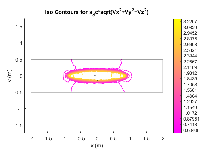


I have tried using "plotgeom" just before (**) and after (***) the "postplot" command:

 
    % plotgeom (PROB, 'parent', f2)       % **
    
    % If want to display iso colors also:
    % postplot( fea2, 'parent', f2, 'surfexpr', 'u', 'isoexpr', 'u' );
    postplot( fea2, 'parent', f2, 'isoexpr', 'u', 'isomap', cmap, 'isolev',...
        lvls, 'title', 'Slice ISO Lines', 'xlabel', 'x', 'ylabel', 'y', 'zlabel', 'z' );
    
    % plotgeom (PROB, 'parent', f2)     % ***

... but these calls seem to interfere with each other.

I wondered about using "geom/plotgeom2" or "geom/plotgeomb" but they did not seem to be on the path.  Before I added "geom/" to the path I though I would just ask for help...... so

Help,
Randal

randress wrote

I would like to add the geometry to the 2D plot such as the one below.
...
I have tried using "plotgeom" just before (**) and after (***) the "postplot" command.

I think it should work with plotgeom, but using postplot might be better to just visualize the geometry edges. I have tried the function call

    postplot( PROB, 'boundary', 'on', 'surfexpr', 0, 'facecolor', 'none', 'colorbar', 'off', 'axis', 'off' );
    postplot( fea2, 'parent', f2, 'isoexpr', 'u', 'isomap', cmap, 'isolev',...
              lvls, 'title', 'Slice ISO Lines', 'xlabel', 'x', 'ylabel', 'y', 'zlabel', 'z' );
    view(2)

using one of your previously attached models "cylinders_between_cylinders_in_boxv1.fea" and the command

    isolineslice( fea, "s_dc*sqrt(Vx^2+Vy^2+Vz^2)", "XY", 0.5, 40, "jet" )

with seems to work as intended.


As a side note, although it probably has nothing to do with this issue, I would suggest to avoid using the Matlab string type defined by double quotation marks ("string_string") in favor of the old single quote char type ('char_string'). At least for any inputs to FEATool function calls (such as postplot) as the string type is not backwards compatible and hence may not be handled properly everywhere (by FEATool functions). This also means that you can not use the following form (my_str == "my_string") to test for string (in-)equality, but must use either strcmp(my_str,'my_string') or isequal(my_str,'my_string') (as == with chars returns a logical array with one entry for every character). I have introduced functionality to try to catch and convert input strings to chars but this may not catch all possible cases.

Precise Simulation wrote

I think it should work with plotgeom, but using postplot might be better to just visualize the geometry edges. I have tried the function call

    postplot( PROB, 'boundary', 'on', 'surfexpr', 0, 'facecolor', 'none', 'colorbar', 'off', 'axis', 'off' );
    postplot( fea2, 'parent', f2, 'isoexpr', 'u', 'isomap', cmap, 'isolev',...
              lvls, 'title', 'Slice ISO Lines', 'xlabel', 'x', 'ylabel', 'y', 'zlabel', 'z' );
    view(2)

I am sure the geometry outline will be just what I was looking for.  Thanks!

Precise Simulation wrote

As a side note, although it probably has nothing to do with this issue, I would suggest to avoid using the Matlab string type defined by double quotation marks ("string_string") in favor of the old single quote char type ('char_string'). At least for any inputs to FEATool function calls (such as postplot) as the string type is not backwards compatible and hence may not be handled properly everywhere (by FEATool functions). This also means that you can not use the following form (my_str == "my_string") to test for string (in-)equality, but must use either strcmp(my_str,'my_string') or isequal(my_str,'my_string') (as == with chars returns a logical array with one entry for every character). I have introduced functionality to try to catch and convert input strings to chars but this may not catch all possible cases.

I do appreciate your pointing this out. IIRC, as I was tinkering with this script I began using single quotes (since that is how I saw that parameter passing implemented elsewhere), but I was having "is(not)equal" trouble (did not think of using c-like function calls...)  Any and all such corrections, comments, and suggestions, including those related to style, are greatly appreciated.

Kind regards,
Randal

When I attempted to add the suggested modification to isolineslice.m here is what I came up with:

isolineslice2.m

and when I ran it against the result in the fea file in your reply "cylinders_between_cylinders_in_boxv1.fea" using he command:

>> isolineslice2 ( fea, "s_dc*sqrt(Vx^2+Vy^2+Vz^2)", "XY", 0.5, 40, "jet" )

here is the 2D plot I got:
isolineslice2_2D_plot.png

Where did I go wrong ?
-Randal

When the FEATool GUI is active the plotting commands (postplot, plotgeom, plotgrid ...) will by default use the GUI figure/axes to plot in if no parent handle has been specified, so use the form:

    postplot( prob, 'parent', f, ... )

like in the other plot commands in your isolineslice function, to specify a specific figure/axes to plot in.

Ok. Got it.

Here is the latest script with string types and comparisons corrected to be simple strings, the addition of a parameter to add value coloring along with the 2D contours, 2D geometry boundary displayed, more helpful titles, and a less cluttered colormap/key.

isolineslice.m

Here is an example of each plot type (3D, 2D, 2Dw/color):

>> isolineslice( fea, 's_dc*sqrt(Vx^2+Vy^2+Vz^2)', 'XY', 0.5, 20, 'jet', 0)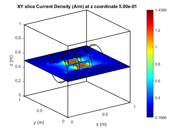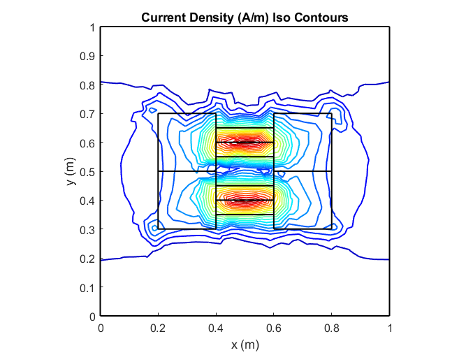

>> isolineslice( fea, 's_dc*sqrt(Vx^2+Vy^2+Vz^2)', 'XY', 0.5, 20, 'jet', 1)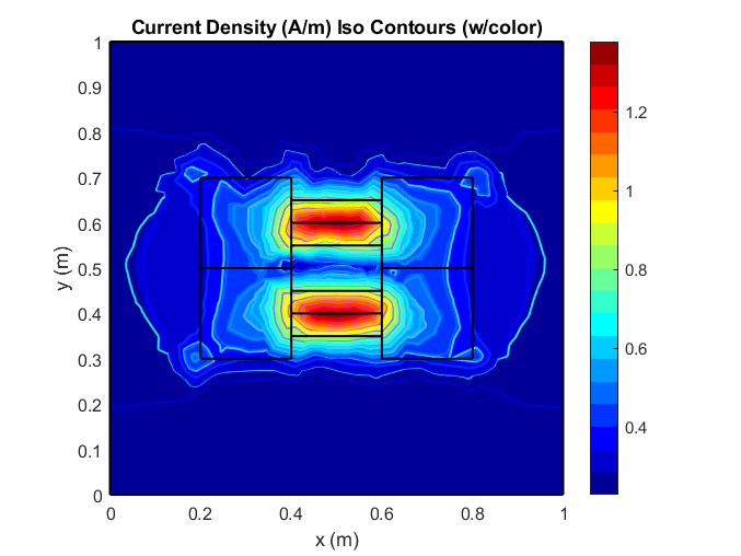

Couple more ideas for this script:

Q1: Is there a call I could make from the script that would save the fea structure from FEATool (same as if I went to FEATool and did File-->Export FEA struct to MATLAB)?

Q2: When I hover over an iso contour near a data point, it displays the coordinates.  How can I get it to display, in addition (or in its place), the value of the data at that point? (see below)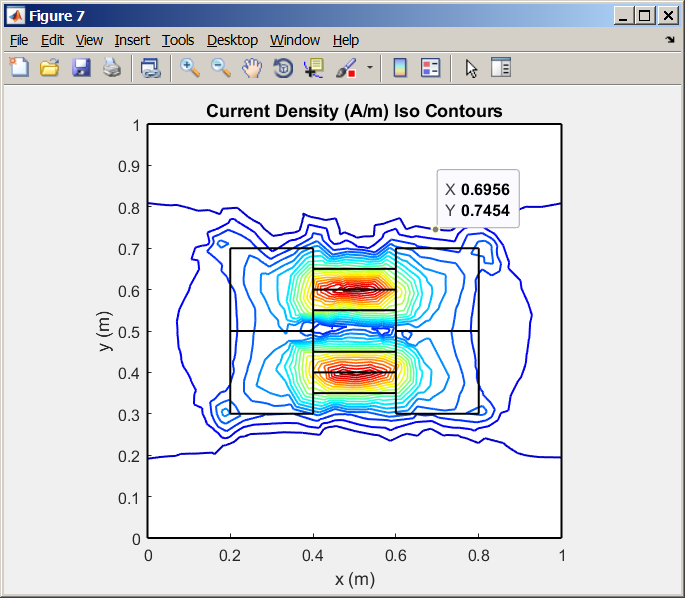



Thanks again,
Randal

randress wrote

Q1: Is there a call I could make from the script that would save the fea structure from FEATool (same as if I went to FEATool and did File-->Export FEA struct to MATLAB)?

This should probably work:

    h_menu_item = findall( 0, 'Label', 'Export FEA Struct To MATLAB' );
    cbf = get( h_menu_item, 'Callback' );
    cbf{1}( h_menu_item, [], cbf{2:end} );

I will probably sooner or later add a custom slice functionality if you get tired of working on this.

randress wrote

Q2: When I hover over an iso contour near a data point, it displays the coordinates.  How can I get it to display, in addition (or in its place), the value of the data at that point? (see below)

You have to create a custom datatip function, for example place/run this code after your plots:

   fcn_datatip = @(~,info) num2str( get(info.Target,'UserData') );
   h_figure = f2; % gcf()
   set( datacursormode(h_figure), 'UpdateFcn', fcn_datatip );

Precise Simulation wrote

This should probably work:

    h_menu_item = findall( 0, 'Label', 'Export FEA Struct To MATLAB' );
    cbf = get( h_menu_item, 'Callback' );
    cbf{1}( h, [], cbf{2:end} );

Indeed it does! (h==>h_menu_item)

I put the code in a parameterless function "export_fea()"
export_fea.m

Precise Simulation wrote

I will probably sooner or later add a custom slice functionality if you get tired of working on this.

... more likely you will grow weary of helping me "tweak" it :-)

Precise Simulation wrote

You have to create a custom datatip function, for example place/run this code after your plots:

   fcn_datatip = @(~,info) num2str( get(info.Target,'UserData') );
   h_figure = f2; % gcf()
   set( datacursormode(h_figure), 'UpdateFcn', fcn_datatip );

Again your suggestion did the job; I substituted sprintf to format the anon function return string and added the coordinates.

nprec = 4;    % add calling argument?

fcn_datatip = @(~,info) sprintf ("%.3e at\n%s %s\n%s %s", ...
    get(info.Target,'UserData'), ...
    xlabel_2D, num2str( info.Position(1), nprec), ...
    ylabel_2D, num2str( info.Position(2), nprec));
h_figure = f2; % gcf()
set( datacursormode(h_figure), 'UpdateFcn', fcn_datatip);

Here is the current version:
isolineslice.m

And here's a call:

>> isolineslice(fea, 's_dc*sqrt(Vx^2+Vy^2+Vz^2)', 'XZ', 0.5, 20, 'jet', 2, 0)

Here is what a 2D figure looks like: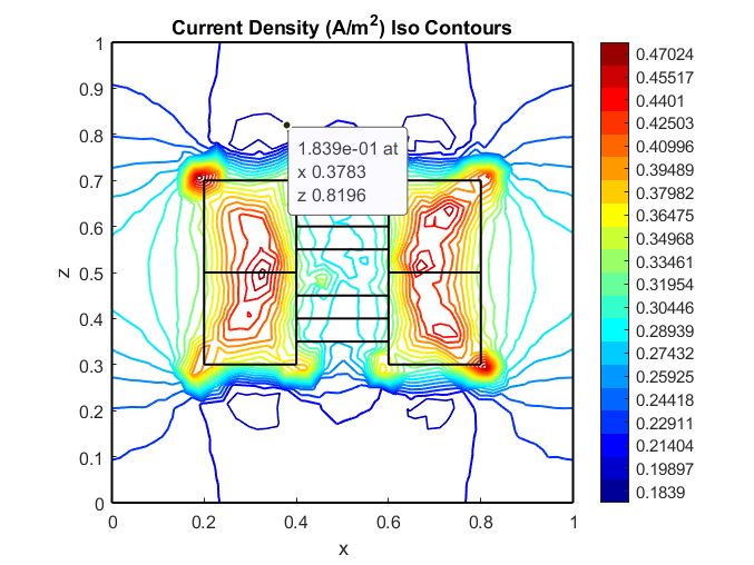


But you can see a bug/anomaly. Notice that the view of the geometry is that perpendicular to the XY plane (from out the z-axis) while the data view is indeed from the specified 'XZ' plane.  

Here's the 3D view which looks correct: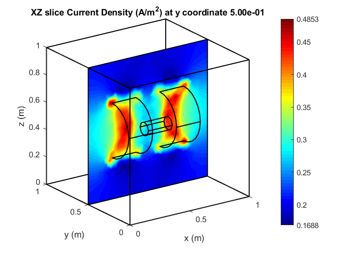


Is the geom going to have to be rotated with the view? How? or is there another way?

Kind regards,
-Randal

randress wrote

I put the code in a parameterless function "export_fea()"

You can also "bypass" the GUI by manually loading the fea struct into the current workspace with:

    load( 'my_model_file.fea', '-mat' )

However, this will naturally prevent you from defining and extracting slices with the GUI, which then must be done programatically.

randress wrote

Notice that the view of the geometry is that perpendicular to the XY plane (from out the z-axis) while the data view is indeed from the specified 'XZ' plane.  

Is the geom going to have to be rotated with the view? How? or is there another way?

Yes, I didn't think about that, the 2D slices will of course always be projected to the xy-plane which when superimposed with a 3D geometry (boundary) will only be correct for z-slices. In other cases you have to rotate the 3D geometry accordingly before you plot it with the postplot command, for example

   fea_rotated = geom_apply_transformation( fea, fea.geom.tags, [], [], pi/2, [1,0,0], [0,0,0] );

will rotate all geometry objects in the fea data struct 90 degrees along the x-axis (vector [1,0,0]) with the base in the point [0,0,0].

Precise Simulation wrote

You can also "bypass" the GUI by manually loading the fea struct into the current workspace with:
 ...

    load( 'my_model_file.fea', '-mat' )

However, this will naturally prevent you from defining and extracting slices with the GUI, which then must be done programatically.

Good to know.  I don't expect I'll be abandoning the GUI to that degree :-)  I suppose that if I had defined a slice before saving the .fea that it might be available.

What I had tried to do was to place conditional code inside "isolineslice.m" and add a flag to its parameter list so that I would have the option of having several "fea" objects in the MATLAB workspace and passing them in vs. getting the one from the problem that is loaded:

function isolineslice (PROB, export_fea_flag, ...)
...
if (export_fea_flag == 1)
   % export fea code
end
...

...but when I tried it, I had what I think were variable existence/scoping issues. When I made the call:

isolineslice (fea, 1 ...)

... if "fea" did not exist in the MATLAB workspace, I got, of course, an error..

But now I am wondering if that would even work since some of what is used by "isolineslice" may be from the loaded model.  Is that correct? 

What I have been doing is going to the GUI File menu to load a previously saved model (which had a slice defined). Then from MATLAB using "isolineslice", plot the three slices (XY, XZ, YZ). That seems to work (except for the boundary rotation for XZ and YZ).

Using the GUI to set it up each time is not a problem.   I'm just glad to be able to get the iso contour line plot!!

Precise Simulation wrote

Yes, I didn't think about that, the 2D slices will of course always be projected to the xy-plane which when superimposed with a 3D geometry (boundary) will only be correct for z-slices. In other cases you have to rotate the 3D geometry accordingly before you plot it with the postplot command, for example

   fea_rotated = geom_apply_transformation( fea, fea.geom.tags, [], [], pi/2, [1,0,0], [0,0,0] );

will rotate all geometry objects in the fea data struct 90 degrees along the x-axis (vector [1,0,0]) with the base in the point [0,0,0].

Well, it would seem to be simple to incorporate this rotation, but I can't seem to get the boundary to move.  I modified the script with a hard coded 'XZ' rotation. Here is my latest attempt:
isolineslice.m
...using this command:

>> isolineslice(fea, 'V', 'XZ', 0.5, 40, 'jet', 2, 0)

... and here are the plots it produced: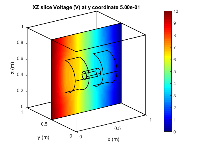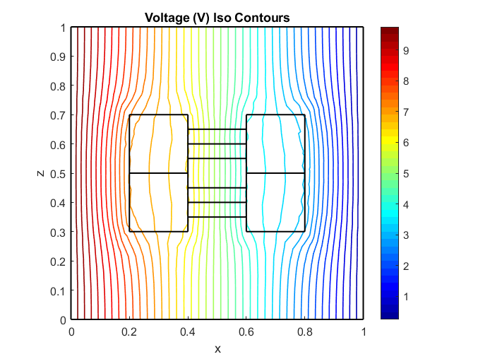




BTW, besides getting more control over the contours themselves (where they stop & start and the interval which is for future tinkering),  I am quite satisfied with the "isolineslice" functionality.  Many thanks for making it happen.

Kind regards,
-Randal

I have now released and updated FEATool to 1.12.3 which amonst other things supports generalized slice plots with the "Post" > "Slice Plot..." menu option, and also includes gradient recovery/reconstruction via L2 projection. Let me know if you find any issues.

randress wrote

...but when I tried it, I had what I think were variable existence/scoping issues. When I made the call:

isolineslice (fea, 1 ...)

... if "fea" did not exist in the MATLAB workspace, I got, of course, an error..

You can test for existing variables with "tf = exist('my_var_name,'var')" and also optional input arguments as "if nargin<5, do_my_setup; end".

randress wrote

But now I am wondering if that would even work since some of what is used by "isolineslice" may be from the loaded model.  Is that correct? 

Whether you are loading the model or exporting from the GUI should result in the same data. What you might be accessing from the Gui is a defined and computed slice.

Precise Simulation wrote

I have now released and updated FEATool to 1.12.3 which amonst other things supports generalized slice plots with the "Post" > "Slice Plot..." menu option, and also includes gradient recovery/reconstruction via L2 projection. Let me know if you find any issues.

WOW! Great news! I had wondered/hoped that your relative silence on the forum meant that you were deep into something of the sort.   I really appreciate it, and I look forward to giving these new features a workout.

Precise Simulation wrote

You can test for existing variables with "tf = exist('my_var_name,'var')" and also optional input arguments as "if nargin<5, do_my_setup; end".
...
Whether you are loading the model or exporting from the GUI should result in the same data. What you might be accessing from the Gui is a defined and computed slice.

That's what I needed to know.  Thanks for the tips.  

Even though I may not need the "isolineslice" with the 1.12.3 release, I think I will go ahead and fix it up as an exercise.

Once again, you have demonstrated that though (and perhaps because) FEATool is not a giant (yet :-) in the FEA s/w arena, your support is second to none!

Kind regards,
Randal

randress wrote

Once again, you have demonstrated that though (and perhaps because) FEATool is not a giant (yet :-) in the FEA s/w arena, your support is second to none!

Kind regards,
Randal

Thank you for the kind words Randal, I really appreciate it. I try my best to help with what I can, let me know of any issues you find.

Johan

Precise Simulation wrote

I have now released and updated FEATool to 1.12.3 which amonst other things supports generalized slice plots with the "Post" > "Slice Plot..." menu option, and also includes gradient recovery/reconstruction via L2 projection. Let me know if you find any issues.

I want to be sure that I understand this enhancement. I had expected something to be different in the "Post Options"/"Postprocessing" GUI form for "Slice Plot", but I find the section to be unchanged.  Correct?

So what I think has been done is that when "Equation Settings" is set to 1st order, that the data for the solution and resultant plot (colorbars) has been subjected to additional processing ("gradient recovery/reconstruction via L2 projection.").  I assume this same data is reflected in the 2D plots produced by such as "isolineslice.m".  Correct?

The only change that I have noticed so far to the "Plot Options" form is the addition of streamlines - which seems to work for me.

In the News forum post you announced:

- Support for boundary and subdomain integral constraints

What I have noticed so far is that these were split into separate forms.  The boundary form (which is what I have interest in) seems to have the added Current Density option. Thanks! I assume that this also taps into the L2 projection gradient recovery data. Correct?  Are there other changes to the boundary surface integration capability?

Precise Simulation wrote

You can test for existing variables with "tf = exist('my_var_name,'var')" and also optional input arguments as "if nargin<5, do_my_setup; end".

I am still having cockpit trouble with this one.  I even tried to incorporate "evalin" to no 'avail'.  I think I will start a separate thread on variable scope and existence. It seems I have a lot to learn :-)

The other item in this thread is the rotation of the geometry issue when the slice is not XY (z-axis). You can see my latest failed attempt in the "isolineslice.m" above.

As always thanks for your help, hints, fixes, and upgrades!

-Randal

randress wrote

I want to be sure that I understand this enhancement. I had expected something to be different in the "Post Options"/"Postprocessing" GUI form for "Slice Plot", but I find the section to be unchanged.  Correct?

Unfortunately, I haven't gotten around to update the documentation yet.

If you load or start a new a 3D model (in FEATool v.1.12.3 Build 20.05.151 or later), there should now be a new "Post" > "Slice Plot..." menu option which allows you to plot general slices which are projected to a 2D plane in a seprate figure that opens, and on this plot you can plot the usual contour, arrow, etc.. plot options (the old slice plot is still available in the usual "Plot Options" dialog box but does not project to a 2D plane). It should look something like the image below.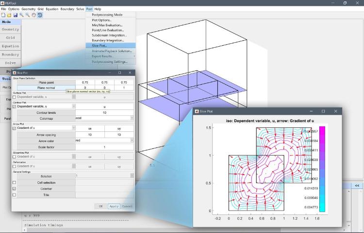

randress wrote

So what I think has been done is that when "Equation Settings" is set to 1st order, that the data for the solution and resultant plot (colorbars) has been subjected to additional processing ("gradient recovery/reconstruction via L2 projection.").  I assume this same data is reflected in the 2D plots produced by such as "isolineslice.m".  Correct?

Not quite I think, what is new is that per default expressions involving first derivatives of dependent variables discretized with first order FEM shape functions will use the L2 projection gradient recovery for postprocessing and visualization. This option can be set in the  "Post" > "Postprocessing Settings..." > "Gradient Smoothing". Note that per default this is only used for 1st order shape functions as it is very expensive for 2nd or higher order shape functions.

randress wrote

In the News forum post you announced:

- Support for boundary and subdomain integral constraints

What I have noticed so far is that these were split into separate forms.  The boundary form (which is what I have interest in) seems to have the added Current Density option. Thanks! I assume that this also taps into the L2 projection gradient recovery data. Correct?  Are there other changes to the boundary surface integration capability?

No, gradient recovery is only used for postprocessing and visualization, not during computation. Or maybe this is a misunderstanding, it will be used for "Post" > "Boundary Integration". However, the new subdomain/boundary integral constraints is found in the "Subdomain" / "Boundary" menus which imposes (mean integral) contstraints on the dependent variable on the solution itself (during computation), and is not related to postprocessing.

randress wrote

I even tried to incorporate "evalin" to no 'avail'.  I think I will start a separate thread on variable scope and existence. It seems I have a lot to learn :-)

Yes, better start a new thread for this.

Precise Simulation wrote

If you load or start a new a 3D model (in FEATool v.1.12.3 Build 20.05.151 or later), ....

Oh... I should have mentioned that I was basing all my comments on 1.12.3.150!  This looks even better ... It's late here so let me chew on 1.12.3.151 a bit the next day or so and I can give a more informed response and address my misunderstandings (which I think will be sorted out a great deal by your reply and seeing 1.12.3.151 in action...

But one quick question. If I open an existing model (build 138 and earlier) will I see the new features OR must it be a NEW model?

Kind Regards,
Randal

Now that I have 1.12.3 build 151, I see the changes and my last comments/questions can pretty much be ignored.  The only ones I wish to reiterate in this thread are:

randress wrote

But one quick question. If I open an existing model (build 138 and earlier) will I see the new features OR must it be a NEW model?

and before that:

randress wrote

The other item in this thread is the rotation of the geometry issue when the slice is not XY (z-axis). You can see my latest failed attempt in the "isolineslice.m" above.

What I would like to do as far as comments/questions regarding the new capabilities of build 151 is to start a new thread(s) and let this one finish up on the 2D plot script issues.

Kind regards,
Randal

randress wrote

But one quick question. If I open an existing model (build 138 and earlier) will I see the new features OR must it be a NEW model?

This should work irrespectively if the model is loaded or genereted from scratch.

randress wrote

The other item in this thread is the rotation of the geometry issue when the slice is not XY (z-axis). You can see my latest failed attempt in the "isolineslice.m" above.

I forgot you are using postplot which actually uses the grid/mesh to visualize the boundary (and everything else). You can see that the geometry has been rotated with "plotgeom", however as the grid/mesh isn't modified "postplot" will show the original boundary. So you would either have to generate a new updated grid using "gridgen" or use "gridrotate" to rotate the grid instead.

Precise Simulation wrote

This should work irrespectively if the model is loaded or genereted from scratch.

The answer I was hoping for ... :-)

Precise Simulation wrote

I forgot you are using postplot which actually uses the grid/mesh to visualize the boundary (and everything else). You can see that the geometry has been rotated with "plotgeom", however as the grid/mesh isn't modified "postplot" will show the original boundary. So you would either have to generate a new updated grid using "gridgen" or use "gridrotate" to rotate the grid instead.

Thanks for the explanation and suggestion.  I will give  "gridgen"and/or "gridrotate" a try.

-Kind regards,
Randal

Precise Simulation wrote

I forgot you are using postplot which actually uses the grid/mesh to visualize the boundary (and everything else). You can see that the geometry has been rotated with "plotgeom", however as the grid/mesh isn't modified "postplot" will show the original boundary. So you would either have to generate a new updated grid using "gridgen" or use "gridrotate" to rotate the grid instead.

I believe I was able to get gridrotate to perform an x-axis rotation for the XZ planar slice and two rotations (y- then z-axis) for the YZ slice (None needed for the XY projection.)

if (isequal(orthoplane, 'YZ'))
 
    grid_rotatedY = gridrotate( PROB.grid, -pi/2, 2);
    grid_rotated   = gridrotate( grid_rotatedY, -pi/2, 3);
    
elseif (isequal(orthoplane, 'XZ'))

    grid_rotated = gridrotate( PROB.grid, -pi/2, 1); 

elseif (isequal(orthoplane, 'XY'))

    grid_rotated = PROB.grid;
else
    error (errmsg);
end
...
PROB.grid = grid_rotated;

I built a wrapper "function isolineslice_ (...)" that implements the solution you offered in another thread "Determining variable scope, existence, and value from a called function" that calls the "function isolineslice(....) after assuring that an fea object is present. It now implements this rotation of the grid/boundary when necessary. Here are the files:
isolineslice_.m

and
isolineslice.m

Thanks for all the help in getting this to be a usable script.  Now with the Slice Plot Post option, I will not use it as much, but I think I will still use it, for example, when trying different parameters (it is very quick and easy to recall the function and change parameters). It should also be userful when wanting to plot different saved fea files in the MATLAB workspace.

Kind regards,
-Randal